The Ultimate Guide to Google Sheets

If you have landed in this blog, I am pretty sure that you are a person who manages reasonably large data and looking for some help in working smart on the Google Sheets. Here is the ultimate guide to Google Sheets where you can learn and explore different capabilities of Google Sheets. Let’s quickly get into it.

What is a Google Sheet?

A Google Sheet is an online application that helps you create, edit, share and modify the data online.

Difference between Excel and Google Sheets

Although Excel and sheets have many similar features, Google Sheets provides links to share with other users to give them permission to read or edit the sheet simultaneously but only one person can edit in Excel.

Creating and Managing Google Sheets

Creating, naming, and saving a sheet

Creating a new sheet from Google Sheets home screen

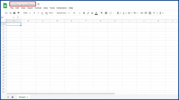
1. Go to the Google Sheets home screen and click the ‘+’ icon.
2. Name the new sheet on the left top corner.
3. The changes you make hereafter will automatically get saved and you can see the document status as saved by clicking the cloud icon on the top.

Creating a new sheet directly from Google Drive

1. Go to Google Drive, click new and choose sheets.
2. You can name and save the sheets as done previously while opening sheets through Google Sheets homescreen.

Copying a spreadsheet

You can copy the spreadsheets by two ways: Method 1: Copying when the sheet is open

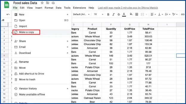
1. Go to the file menu and click “make a copy”.
2. Name the copy of the file, choose the fields, and make a copy..
3. You will get a “copy of the spreadsheet” in the new tab.

Method 2: Copying directly from the Drive

1. Go to Google Drive,right click the file and click “make a copy”.
2. In a few seconds you will get a copy of the original file.

Moving a spreadsheet

You can move the spreadsheet by two ways:

Method 1: Moving when the sheet is open

1. Click the file menu and choose “move”
2. You will get a drop down below the move icon on the top. You can choose the folder you want to move and click ‘move here’.

Method 2: Moving directly from the Drive

1. Go to Google Drive,right click the file and click ‘move’.
2. Follow the same steps as you move the sheet when it is open.

Removing,Deleting, and restoring a spreadsheet

Before I show you how to do it, let me sort the difference. If you remove the file from Drive the file will land on trash and after 30 days it will automatically get deleted. If you delete the file from trash it will be permanently deleted from the Drive.

Removing a spreadsheet : Locate the file on the Google Drive homescreen and drag it to trash.

Restoring a spreadsheet: Go to trash, locate the file, and click ‘restore’.

Deleting a spreadsheet: Locate the file in trash and click ‘delete forever’.

Importing Files

Importing xls and xlsx files

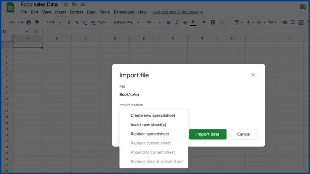
1. Click ‘import’ and choose the file from your device
2. Choose the preferred option from the dialogue box. Hence the file is imported.

Importing data files like csv and txt

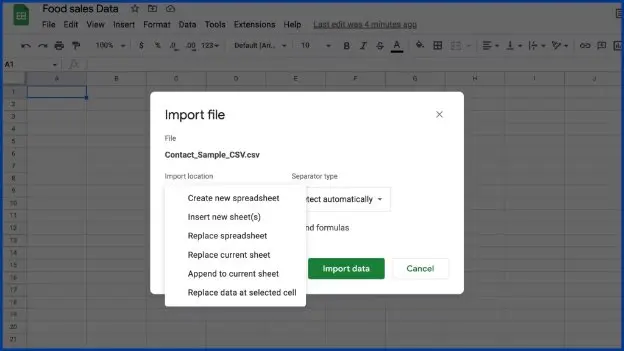
1. Click ‘import’ and choose the file from your device.
2. In the dialogue box choose replace and auto replace formulas.

Editing the Google Sheets

Entering and editing data in cells

• To enter data in an empty cell click the cell and type the text in it.
• To enter data in a cell which has data already, click on the cell and start typing.
• Press “enter” to save the data in the cell.
• Copy and paste data in cells by using “ctrl+c” and “ctrl+v”.
• Use tab key to move the cursor to next cell.
• To fit the data in the cells, select the whole sheet, select one of the column separators, double click and it is done.

Finding and replacing values

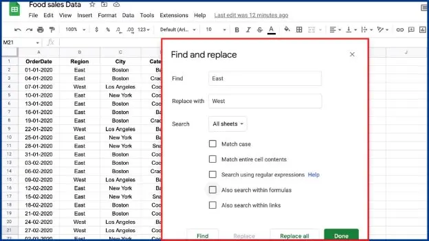
Go to the edit menu, click “Find and replace”, and choose the necessary values in the dialogue box as shown above.

Inserting, deleting, and clearing rows and columns

To insert a column or row: Select a row or column, right click, insert 1 row or column above or below.

To delete a row or column: Select a row or column, right click and choose delete column.

To delete and insert multiple columns and rows: Highlight the columns and rows, right click and delete or insert.

(Tip: When you want to keep the row or column but erase the contents, highlight the rows or columns, right click, and clear the rows or columns.)

Moving or copying rows, columns, and cells

To move rows and columns: Click the particular row or column, drag and drop to the desired location.

To move rows and columns using edit menu: Select the row or columns, go to edit menu, and click move right or left.

To move cells, follow the same process like rows and columns.

(Tip: You can simply use “ctrl+c” to move row, columns, and cells)

Working with multiple sheet

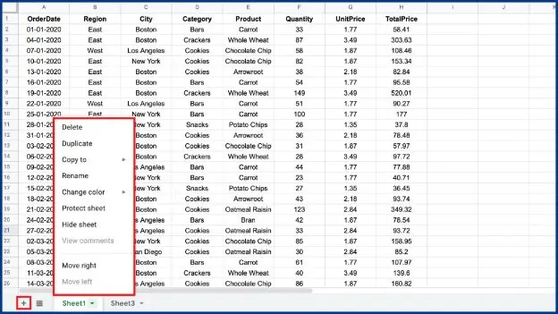
• Click the plus icon at the bottom to add a sheet. Drag and drop the sheets to make it in order or down arrow to move left or right.
• To delete the sheet, click the down arrow and delete the sheet.
• To name or rename the sheet, click on the name, and edit it.
• To make a copy of the sheet, click the small arrow and select duplicate.
• To copy to a new spreadsheet, click the down arrow and copy to a new or existing spreadsheet.
• To change the colors for the icon with sheet name, click the small arrow and choose your desired colors.

Creating a series of numbers, letters, or dates

• Enter at least two instances and drag it with the left right corner.
• To enter a series of dates in a row or column, follow the same process above.

Inserting images and hyperlinks

To insert a floating image:(image8)

1. Select a cell, go to the insert menu and choose “image over cells”.
2. Browse the image, resize and place it on the sheet accordingly.

To insert an image within a cell, follow the same steps and choose “image in a cell” option instead of “image over cells”.

To hyperlink the text in sheet: Select the cell or text, go to the insert menu, choose link, paste it and click ok.

Viewing the spreadsheets

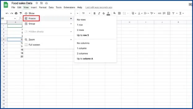
Freezing rows and columns

1. Select a row or column.
2. Go to the view menu.
3. Freeze the desired number of rows or columns

Hiding rows, columns, and sheets

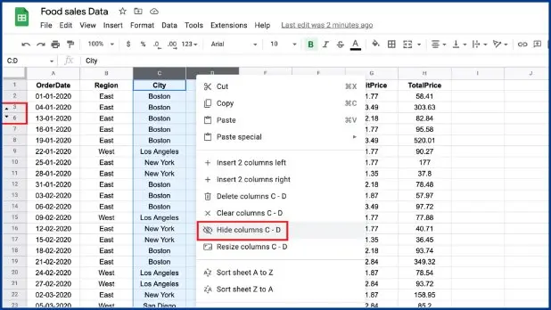
1. Select the rows or columns.
2. Right click and choose hide.
3. Click the arrows near the hidden rows or columns to unhide it.

Using filters and creating filter views

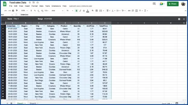
1. Select the columns, choose the filter option, click the filter icon on the filtered columns and filter it accordingly.
2. Go to the data menu and choose the “save as filter” option.
3. The filter view is now viewed as dark gray and the name can be edited.
4. Click the “X” icon, close the filter, and deselect the filter icon to return back to the original sheet.
5. To return to the filtered sheet, click the drop down near the filter icon and open the file.

Sorting data on a spreadsheet

Sorting a particular column

1. Freeze the labels of the column if needed.
2. Select the small drop down on the top of the particular column and sort a-z or z-a.

Sorting multiple columns, Select the entire sheet, go to data menu and choose sort range.

Formatting the spreadsheets

Formatting cells, rows, and columns

To format currencies: click “$” icon or go to the format menu, choose “number” and click custom currency. Hence you can choose the desired currencies.

To format percentage: click “%” icon or go to the format menu, choose number and click percentage.

Using conditional formatting

1. Go to the format menu and select conditional formatting
2. Fix the range, format rules, font (size, style, and color) and click done

Printing a spreadsheet

1. Go to the file menu and select print.
2. Fix the papersize, scale and margins as per your requirement.
3. Go ahead with printing.

Working with data on Google Sheets

Sum, Average, Min, Max, or Count

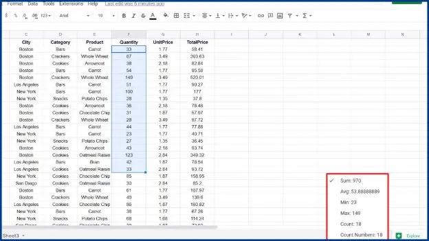
• Select the particular row and see the sum, avg, and more in the bottom button.
• For non adjacent columns view the Sum, Average, Min, Max, or Count by using ctrl key and selecting the required fields.

Using formulas and functions

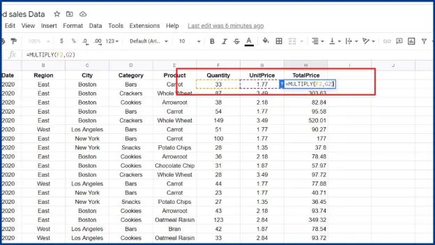
1. Click the view menu and select the formula bar.
2. Use the ‘multiply’ function for the first row.
3. Drag to the whole column if you want to apply the same formula for the entire column. (similarly you can perform other functions in sheets)

Using IF and nested functions in formulas

If function:

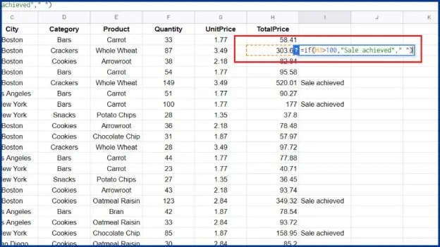
An ‘if’ function is used to make logical comparison between a value and your expected outcome whether it is true or false.

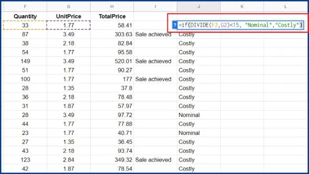
Here is an example of an ‘if’ function” where I want to see the dates during which the sale exceeds 100.

Nested function:

A nested function is performing a function within a function.

Here is an example where I want to mark the commodity as costly if the unit price is greater than 15. Hence I am using ‘division’ within ‘if function.

Creating charts and graphs

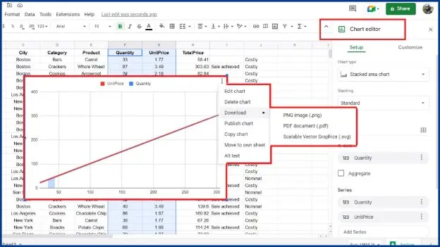
1. Select data and click graph icon on the top.
2. Google Sheets auto generates a chart.
3. Now customize the chart using the chart editor.

Using pivot table

1. Click the data menu and create a pivot table.
2. A pivot table will be created on the existing or new spreadsheet.
3. Select the customized options in the pivot table editor.
4. Hence the pivot table is created.

Collaborating with Google Sheets

Sharing the spreadsheet with other people

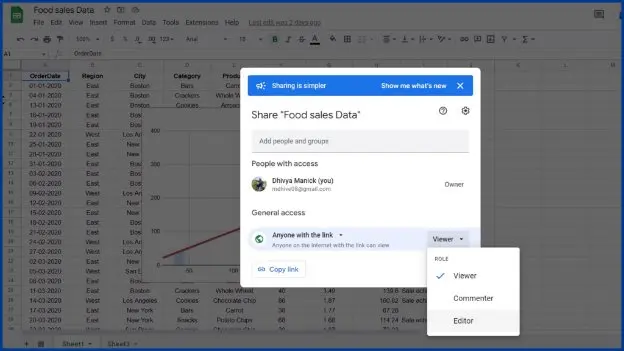
1. Click the share button on the top right corner.
2. Enter the email address of the people you want to share in the opened dialogue box.
3. Select the permission options, add a message if you wish and you can share the spreadsheet.
4. You can also share the sheet with anyone by choosing the option ‘anyone with link’.

Publishing the sheet on web

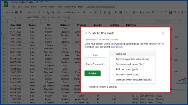
1. Go to the File menu, click share and choose publish to the web.
2. Choose the format to be published and click publish.

Commenting on a spreadsheet

Click the profile picture of the collaborator in the top right corner and you can comment on them. You can also group chat by clicking the chat button on the top.

Spreadsheet revisions

You can see the version history of the sheet by clicking on the notification displayed next to the help menu.You can restore a particular version by clicking ‘restore this version’. The restoration process does not destroy any versions of the spreadsheet. It simply restores and adds that version. You can always go back to the revised version of the document by opening version history again and restoring that version.

I hope the above blog showcasing the ultimate guide to Google Sheets has helped you to work on Google Sheets faster and smarter. If you have any help or queries on Google Sheets kindly let us know in the comment section.